2026
CRAN-PM
A dual-branch Vision Transformer for daily PM2.5 forecasting at 1 km resolution across Europe. 29 million pixels in 1.8 seconds. Zero-shot transfer to USA, Canada, and India.
A dual-branch Vision Transformer for daily PM2.5 forecasting at 1 km resolution across Europe. 29 million pixels in 1.8 seconds. Zero-shot transfer to USA, Canada, and India.
Abstract
Vision Transformers have achieved remarkable success in spatio-temporal prediction, but their scalability remains limited for ultra-high-resolution, continent-scale domains required in real-world environmental monitoring. A single European air-quality map with 1 km resolution comprises 29 million pixels, far beyond the limits of naive self-attention.
We introduce CRAN-PM, a dual-branch Vision Transformer that leverages cross-resolution attention to efficiently fuse global meteorological data (25 km) with local high-resolution PM2.5 at the current time (1 km). We further introduce elevation-aware self-attention and wind-guided cross-attention to force the network to learn physically consistent feature representation for PM2.5 forecasting.
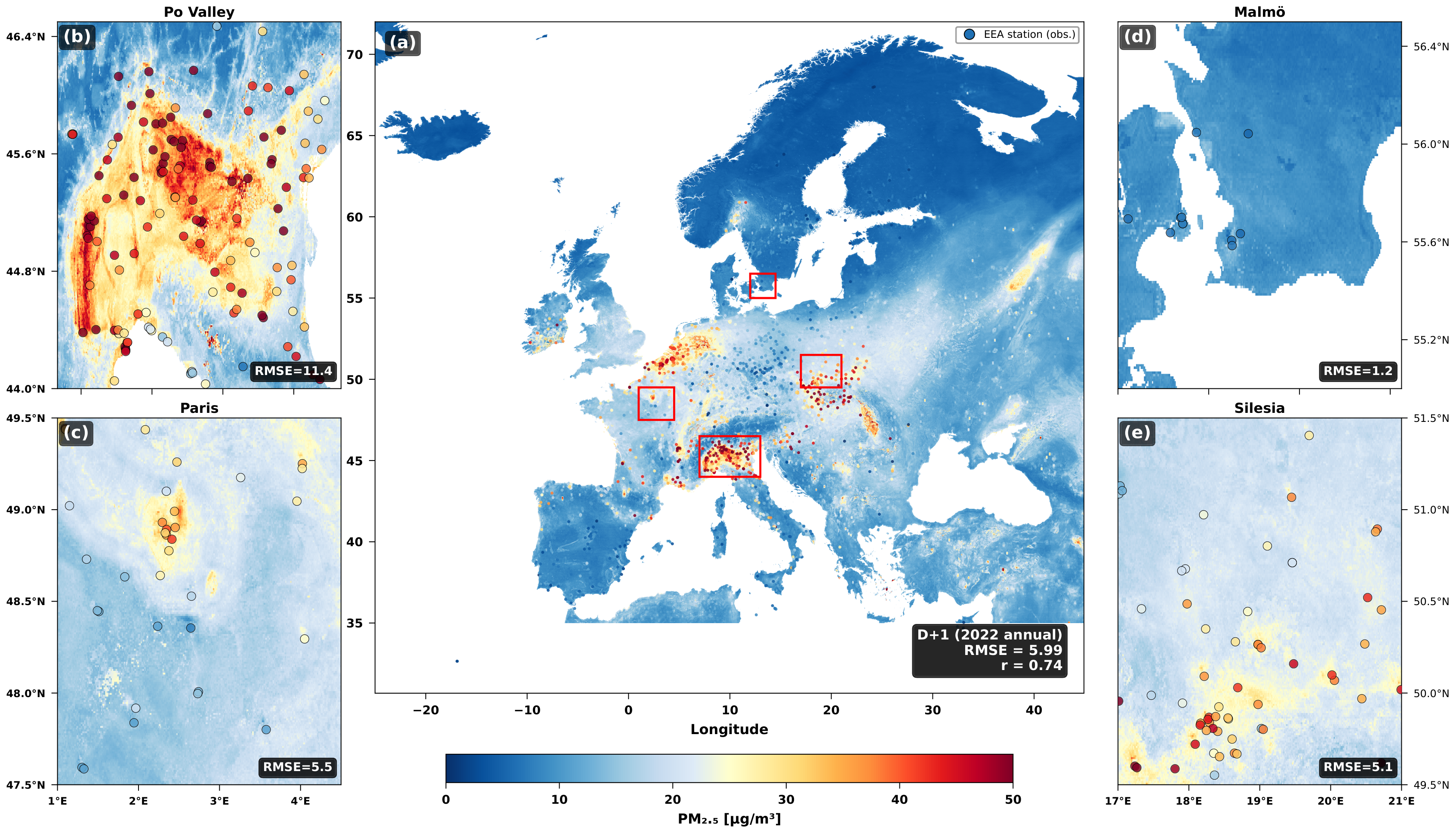
CRAN-PM is fully trainable and memory-efficient and generates the complete 29-million-pixel European map in 1.8 seconds on a single GPU. Evaluated on daily PM2.5 forecasting throughout Europe in 2022 (362 days, 2,971 stations of the European Environment Agency), it reduces RMSE by 4.7% at T+1 and 10.7% at T+3 compared to the best single-scale baseline, while reducing bias in complex terrain by 36%.
Interactive
Four interactive visualisations of the core mechanisms behind CRAN-PM.
A PM2.5 map is tokenised at two resolutions. The global branch creates coarse 25 km patches; the local branch splits fine 1 km tiles. Cross-attention bridges the gap.
Attention is biased toward upwind sources via a learnable wind alignment score. Upwind tokens receive higher attention weights.
An asymmetric ReLU bias penalises attention to higher-elevation sources. Pollution flows downhill (katabatic) but is blocked uphill.
Fused tokens are reshaped to 32×32 then progressively upsampled through 4 PixelShuffle stages to the final 512×512 resolution. Watch pixels unfold.
Global tokens are reordered based on wind direction so the transformer processes upwind patches first. Patches physically move to new positions — watch how the scanning order changes with wind.
Architecture
A global branch processes coarse meteorology while a local branch encodes fine-scale PM2.5 and elevation. Wind-guided cross-attention bridges the 25× resolution gap.
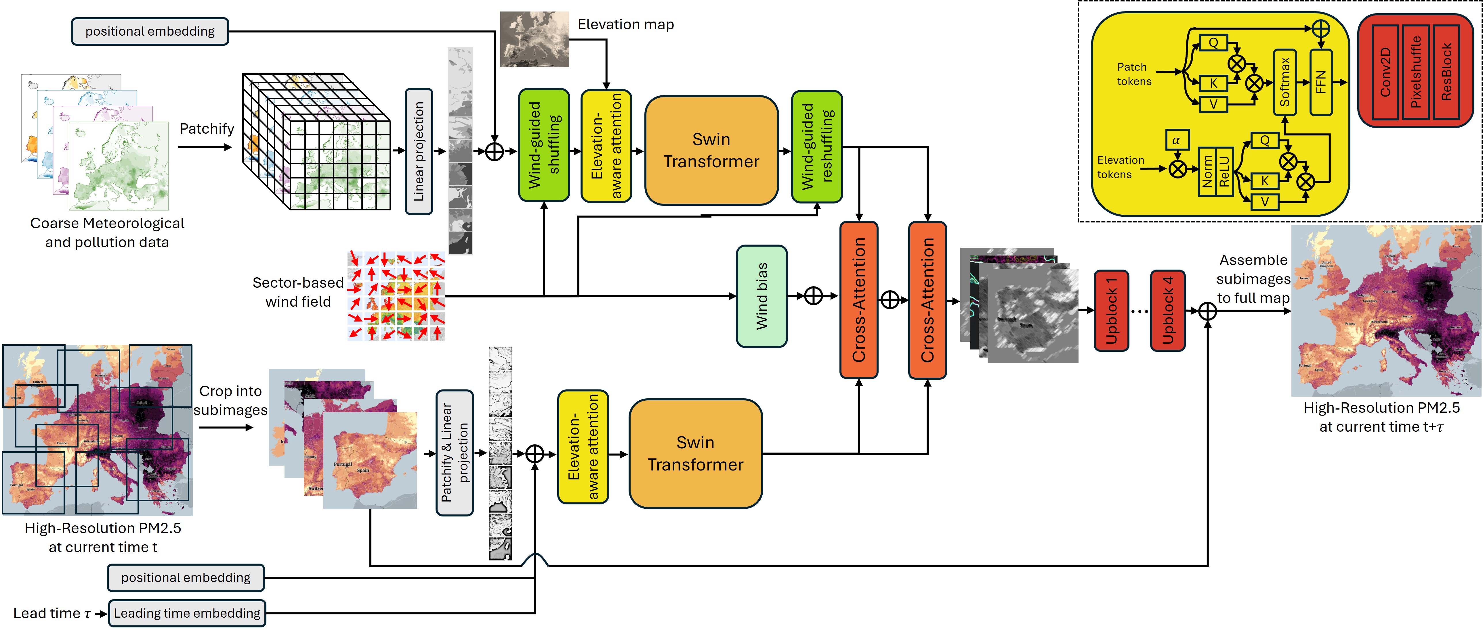
Figure 2. A global branch (top) encodes coarse meteorological fields with wind-guided token reordering and elevation-aware attention; a local branch (bottom) encodes high-resolution PM2.5 subimages. Two wind-biased cross-attention layers fuse the branches (fine queries coarse). A PixelShuffle-based decoder reconstructs the residual, and subimage predictions are reassembled into the full European map.
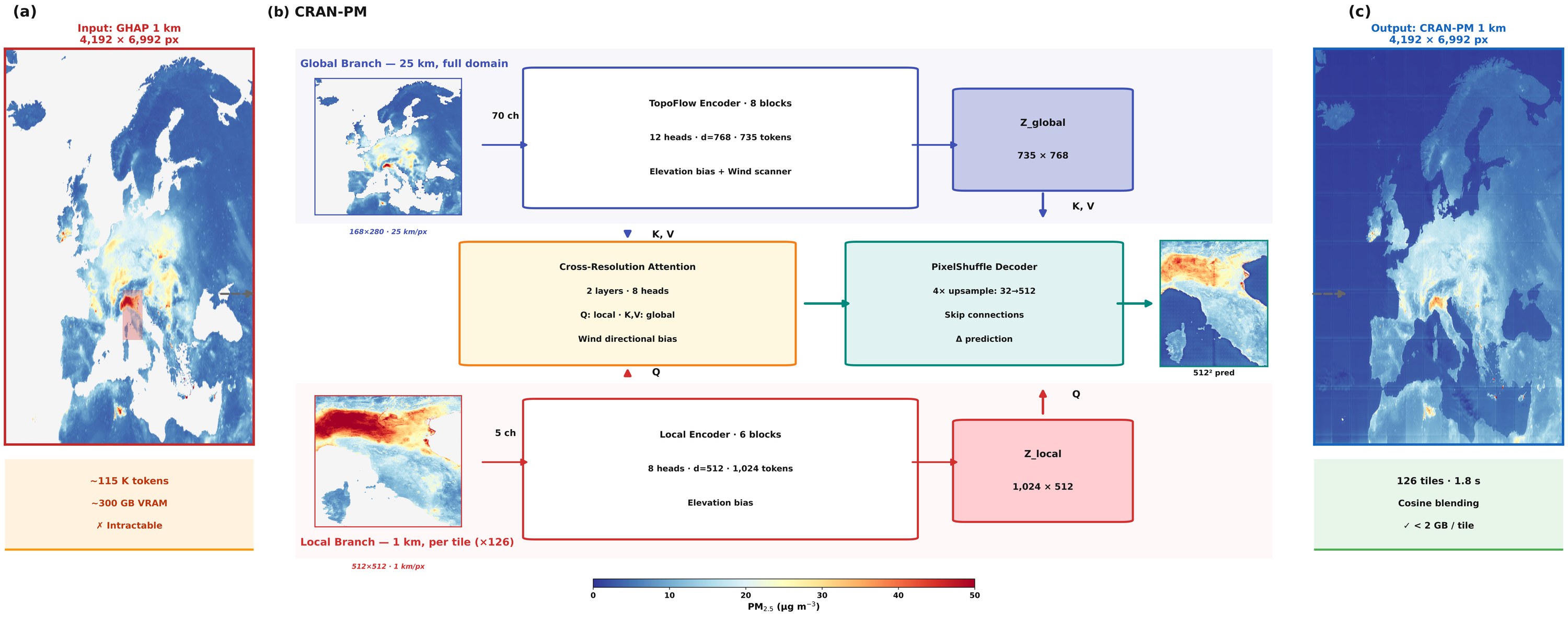
Figure 7. CRAN-PM architecture overview showing the elevation-aware attention mechanism (yellow inset) and the data flow between global and local branches.
Method
Four design choices that enable high-resolution air quality prediction from coarse inputs.
Local fine-resolution tokens (1 km) query global coarse tokens (25 km) for large-scale meteorological context. A wind-guided bias aligns attention to upwind sources, reflecting the causal physics: local PM2.5 responds to global meteorology, not vice versa.
Instead of predicting absolute PM2.5, the decoder outputs a residual Δ added to today's observation. Zero-initialised final convolution ensures the model starts at the persistence baseline, dramatically stabilising early training.
Fused local tokens are reshaped to 512×32×32, then four PixelShuffle upsampling blocks progressively restore 512×512 resolution (512→256→128→64→32 channels). Each block: convolution + PixelShuffle + residual block. Prevents checkerboard artifacts.
An asymmetric ReLU bias penalises attention to higher-elevation sources while leaving downhill interactions unaffected, consistent with katabatic flows. Injected as an architectural prior in the first attention block of each branch.
Results
CRAN-PM evaluated on the held-out 2022 test set at 1 km resolution over all of Europe.
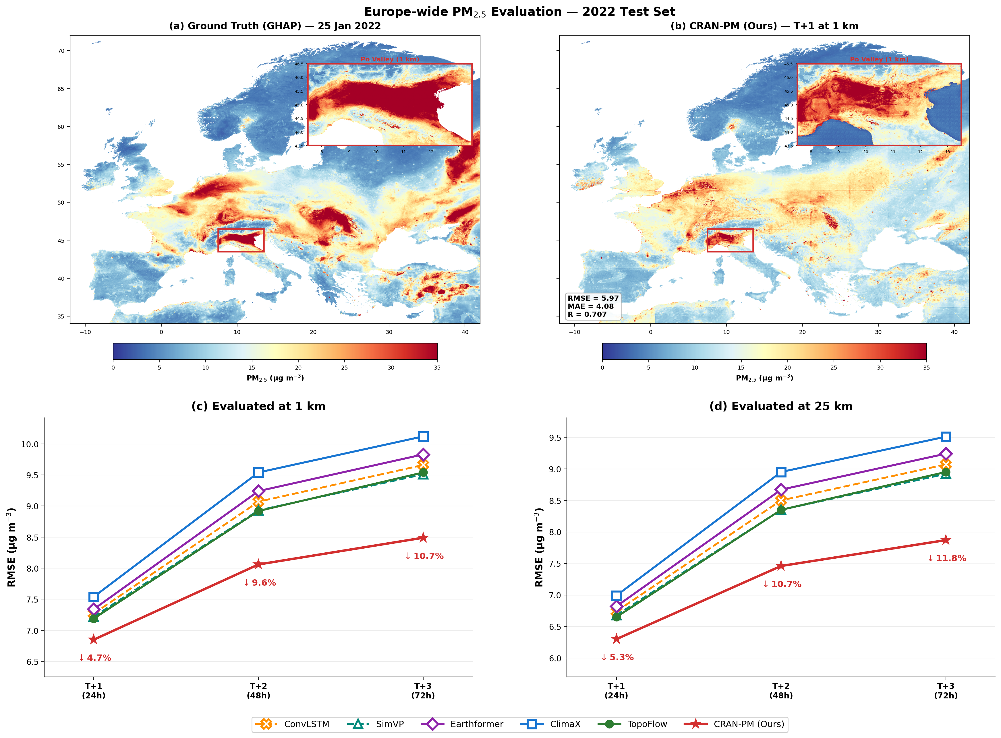
Figure 3. (a) Ground truth (GHAP, 1 km) for January 25, 2022. (b) CRAN-PM T+1 prediction at 1 km; inset shows the Po Valley zoom. (c, d) RMSE degradation across forecast horizons T+1 to T+3, evaluated at 1 km and 25 km. CRAN-PM consistently outperforms all baselines, with the gap widening at longer horizons.
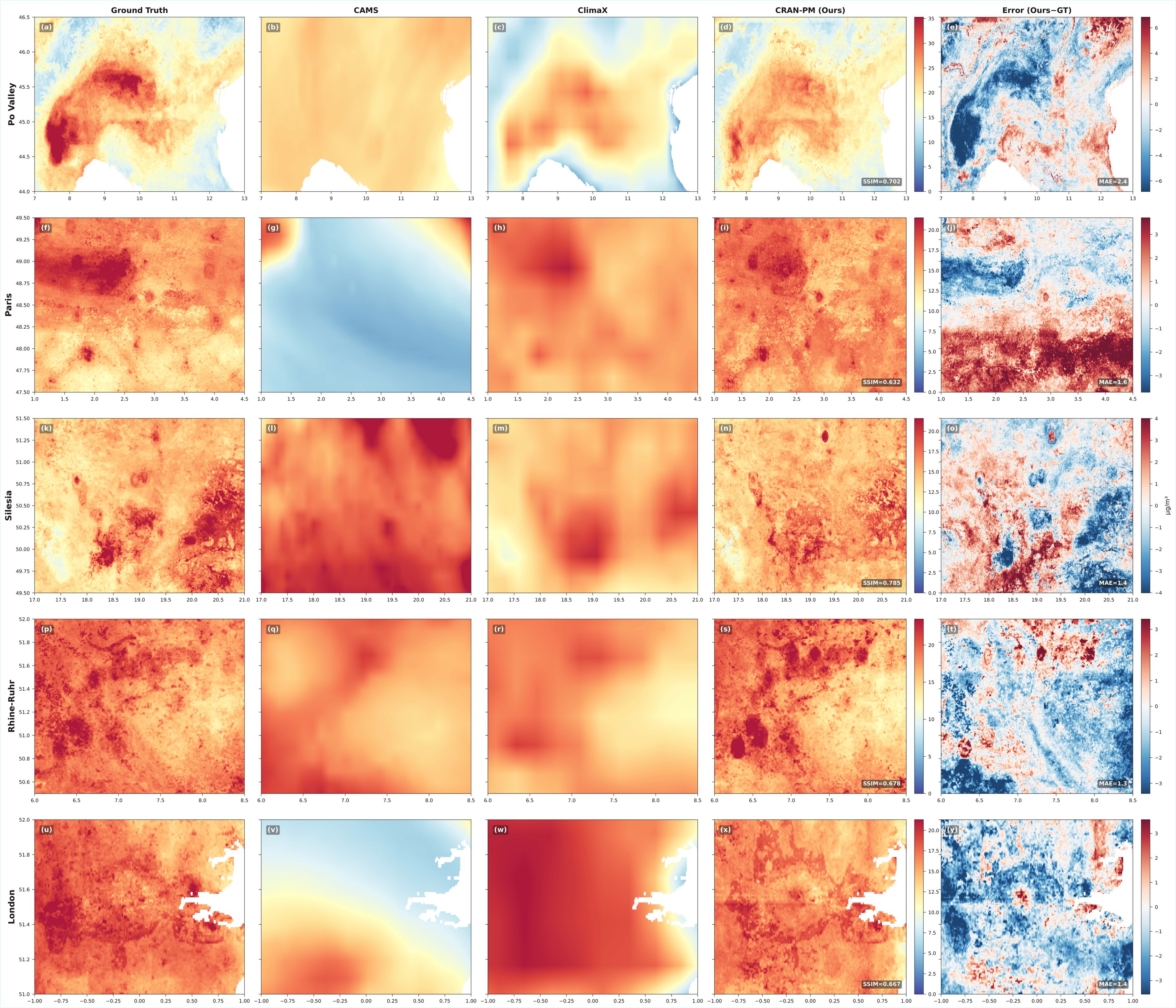
Figure 4. Five regions (rows): Po Valley, Paris, Silesia, Rhine-Ruhr, London. Columns: (a) ground truth, (b) CAMS, (c) ClimaX, (d) CRAN-PM, (e) error (ours − GT). CAMS produces overly smooth fields; ClimaX shows blocky 25 km artifacts; CRAN-PM recovers fine-grained spatial structure with SSIM ≥ 0.63 across all regions.
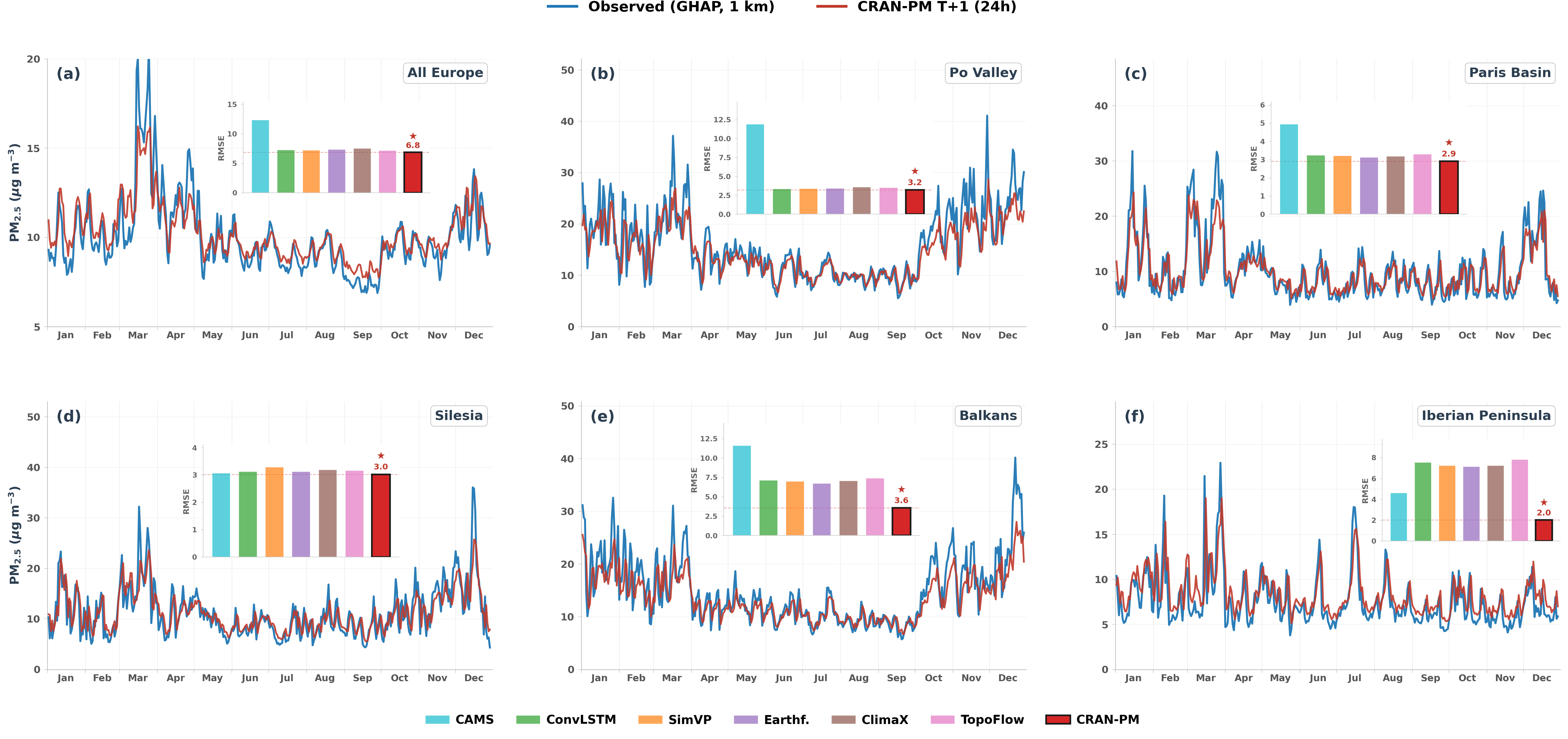
Figure 5. Blue: observed (GHAP, 1 km); red: CRAN-PM prediction. (a) All Europe, (b) Po Valley, (c) Paris Basin, (d) Silesia, (e) Balkans, (f) Iberian Peninsula. Inset bar charts compare regional RMSE across all methods; CRAN-PM (dark red) achieves the lowest error in all regions.
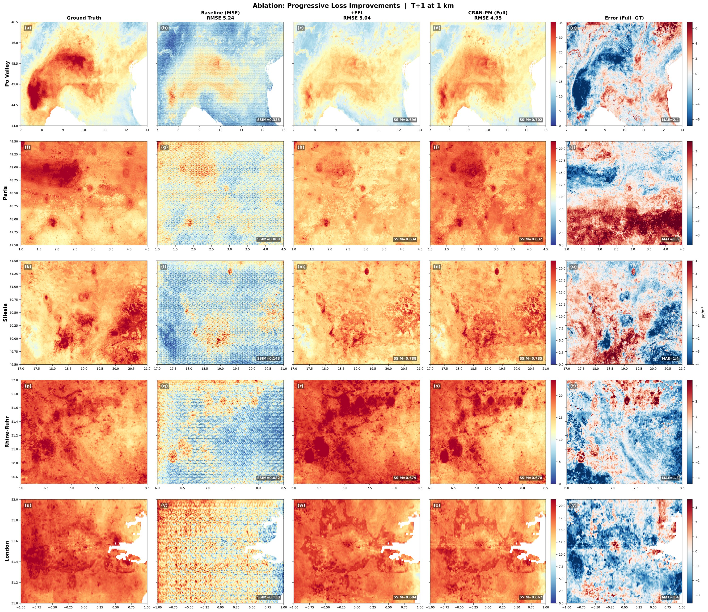
Figure 6. Five regions (rows): Po Valley, Paris, Silesia, Rhine-Ruhr, London. Columns: (a) ground truth, (b) baseline (MSE only, RMSE = 5.24), (c) +FFL (RMSE = 5.04), (d) CRAN-PM full (RMSE = 4.95), (e) error (full − GT). The baseline produces blurred outputs (SSIM ≤ 0.34); FFL dramatically recovers spatial structure; station loss further reduces systematic bias.
Zero-Shot Transfer
Trained only on Europe, CRAN-PM transfers zero-shot to unseen continents — capturing wildfire plumes and pollution hotspots without any fine-tuning.
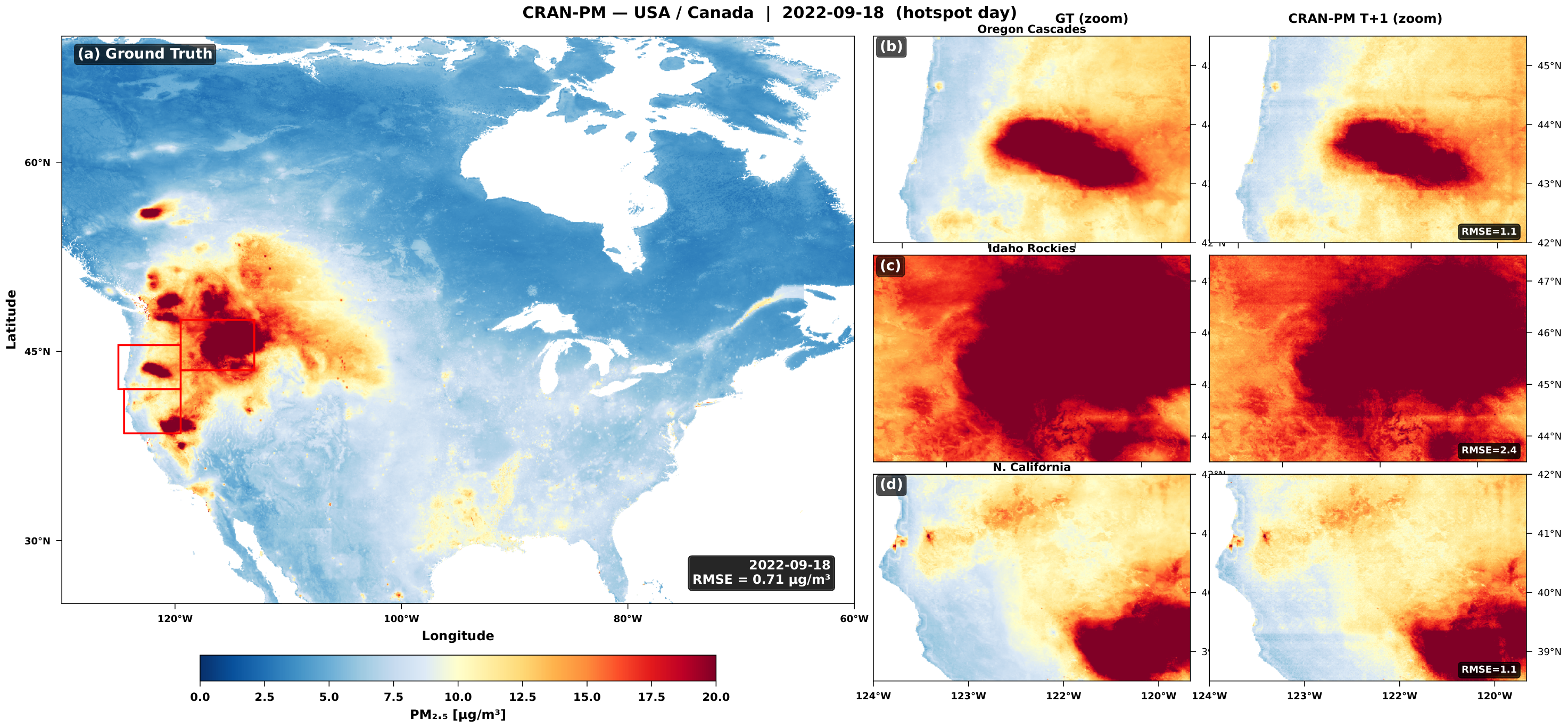
Figure 8. Zero-shot prediction during a major wildfire episode. CRAN-PM identifies the smoke plume extent and intensity despite never seeing North American geography during training.
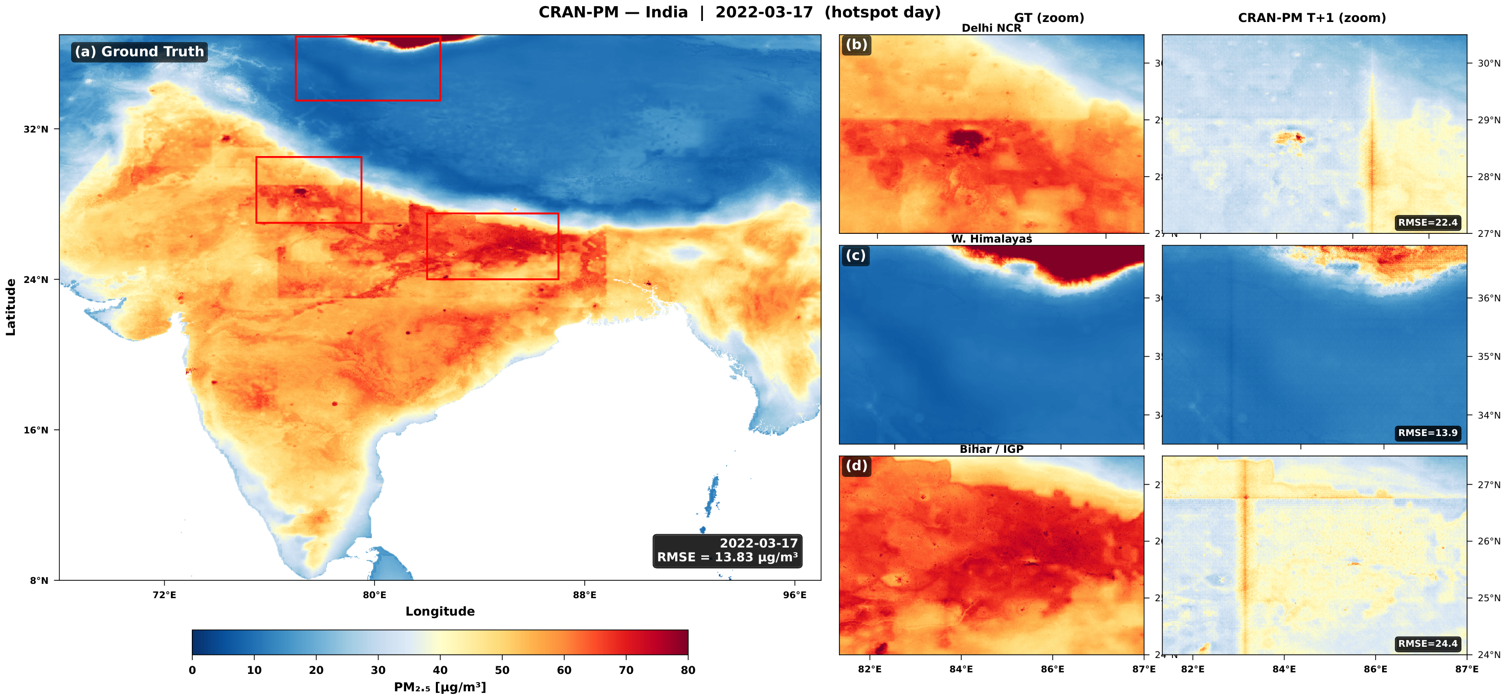
Figure 9. Zero-shot transfer to India capturing the persistent pollution belt across the Indo-Gangetic Plain. The model resolves the sharp gradient at the Himalayan foothills where pollutant transport is blocked by topography.
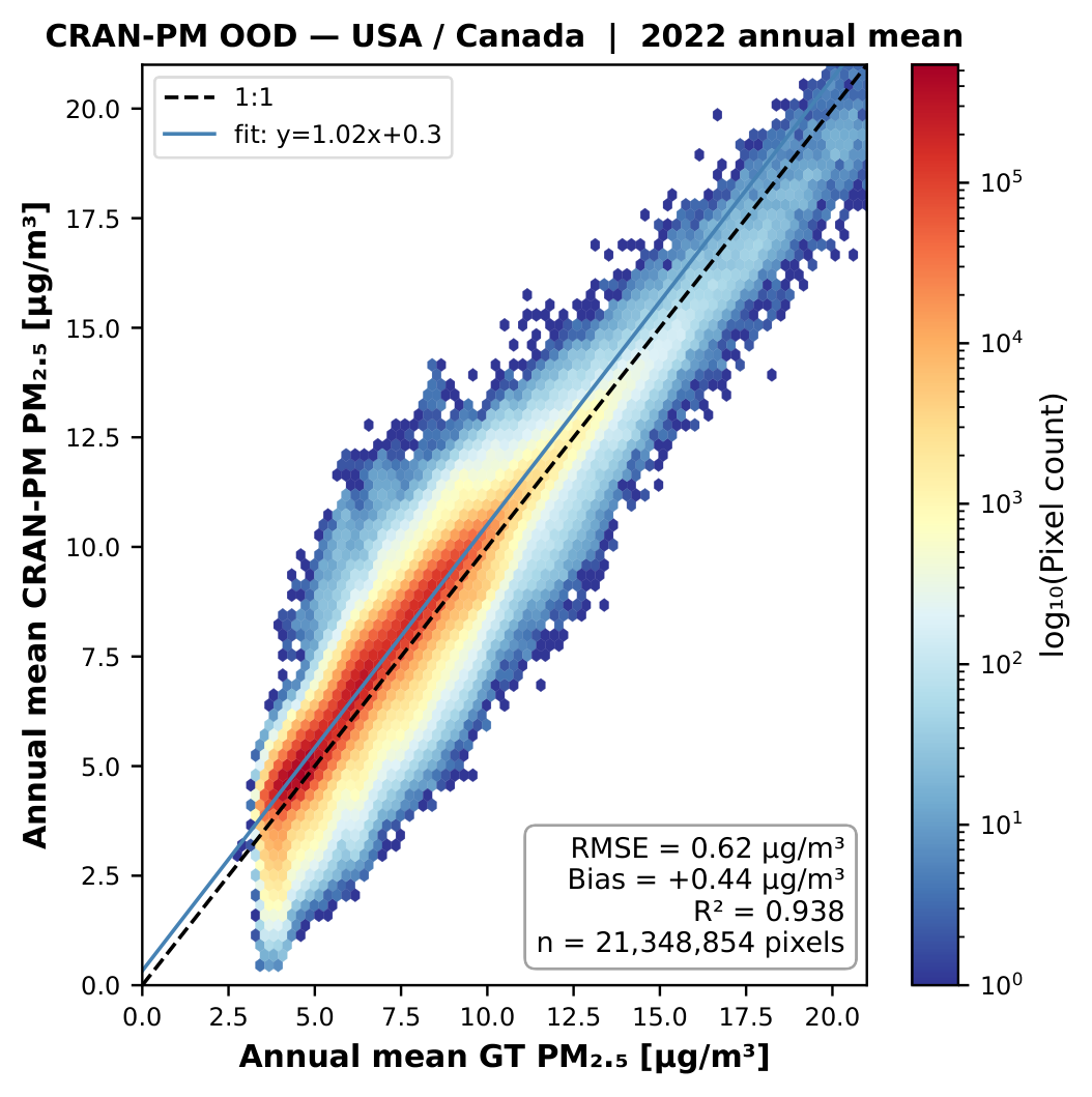
Figure 10a. Density scatter plot of predicted vs. observed annual mean PM2.5 for the USA/Canada domain (2022).
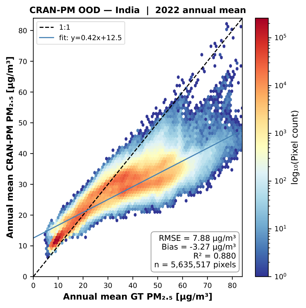
Figure 10b. Density scatter plot for the India domain (2022). Despite extreme PM2.5 levels (>150 μg/m³), CRAN-PM maintains strong correlation without fine-tuning.
Specifications
Architecture parameters and training configuration for reproducibility.
| Architecture | |
|---|---|
| Global Input | ERA5 + CAMS, 0.25°, 70 channels |
| Local Input | GHAP + elev/lat/lon, 0.01°, 5 channels |
| Global Patches | 168 × 280 → 735 tokens (patch 8) |
| Local Patches | 512 × 512 → 1,024 tokens (patch 16) |
| Global Dim / Depth | 768 / 8 blocks (1 elev-aware + 7 Swin) |
| Local Dim / Depth | 512 / 6 blocks (1 elev-aware + 5 Swin) |
| Cross-Attention | 2 layers, 8 heads, dim 64 |
| Decoder | 4-stage PixelShuffle |
| Full Map | 4,192 × 6,992 (126 tiles) |
| Parameters | 96M |
| Training | |
|---|---|
| Optimizer | AdamW (β1=0.9, β2=0.999) |
| Learning Rate | 5e-5 (cosine decay) |
| Batch Size | 32 (gradient accumulation) |
| Precision | bfloat16 mixed |
| Epochs | 30 (5-epoch warmup) |
| Train Period | 2017–2021 |
| Test Period | 2022 |
| Loss | MSE + FFL + Station (λ=0.1) |
| Hardware | 64× AMD MI250X (LUMI-G) |
| Framework | PyTorch + DDP |
| Data Source | Resolution | Variables |
|---|---|---|
| ERA5 | 0.25° | 60 ch: surface + 5 pressure levels (t & t−1) |
| CAMS Analysis | 0.25° | 10 ch: PM2.5, PM10, NO2, O3, CO (t & t−1) |
| GHAP | 0.01° | PM2.5 satellite-derived (t & t−1) |
| SRTM | ~1 km | Elevation + lat/lon |
Quick Start
Install and train CRAN-PM in a few commands.
Citation
If you find CRAN-PM useful, please cite our paper.
@inproceedings{kheder2026cranpm,
  title     = {Cross-Resolution Attention Network for
               High-Resolution {PM}$_{2.5}$ Prediction},
  author    = {Kheder, Ammar and Toropainen, Helmi and
               Peng, Wenqing and Ant{\~a}o, Samuel and
               Liu, Zhi-Song and Boy, Michael},
  booktitle = {Proceedings of Computer Vision Conference},
  year      = {2026}
}